The LatticeRobot Unit Cell Parameter System

We are thrilled to share LatticeRobot to help index and inventory the useful properties of lattices and other mesoscale structures, textures, and metamaterials. To attempt this content aggregation challenge raises questions of data organization and presentation. Although we intend to create an environment where data speaks first and engineers can discover useful lattice systems that deliver known functionality, there are several organizational and naming systems used across academia and industry to reconcile and reference. Most naming conventions describe individual objects like diamond and gyroid TPMS, yet these simple cases of more general periodic functions. Also, various periodic structures, despite having very different constructions and parameterization, such as the simple cubic beam and the implicit approximation of the Schwarz (P) TPMS lattice, are geometrically and mechanically very similar. We can aspire to make all of this data navigable, but what's the one true way to write it all down?

First, let's scope the problem to implicit descriptions of geometry. Implicit modeling for lattice design in engineering has proven to be a robust method to capture the mesoscale, and most CAD and generative systems are starting to embrace implicits. If all of our unit cells and representative volume elements are modeled by fields, the fields themselves are the ultimate descriptors of their functionality. Perhaps we could organize the parametric families by examining the structure of the fields via simple functional analysis. Perhaps we could use this structure to bridge between different kinds of lattices like the simple cubic and the Schwarz, despite being made of very different functions.

What is an implicit model or a signed distance field?

Let's quickly get familiar with the idea of representing a shape like a lattice with an implicit function of which a signed distance field ("SDF") is a common special case. We will write down some function F(p) that evaluates any position p in space, and define:

• F(p) < 0: p is inside the shape;
• F(p) = 0: p is inside the shape; and
• F(p) > 0: p is outside the shape.

We can offset outward by subtracting from our function and use other functions to modify the shape we're representing. Boolean operations, for example are often handled by min and max functions.

Periodic functions in one dimension

In engineering, we tend use the word "periodic" to refer to repeating structures, even when they vary. Implicit models can often represent these structures efficiently. Let's look at some one-dimensional periodic structures to get a feel for how they make shapes by comparing a triangle wave to sine or cosine wave. In this case, our one-dimensional solids are the vertical bands on the x axis.

Any intuition you might have about time-dependent waveforms from signal processing or analogue sound synthesis carries over to our spatially parameterized models, and we borrow terminology like "bias" and "period". It is reasonable to think of the beam or foam lattice as a triangle wave and the Schwarz as a sine wave, as indeed the latter is just the sum of the sines of the three spatial axes:

Schwarz(x, y, z) = cos(x) + cos(y) + cos(z)

The similar-looking blended beam lattice is merely three unioned cylinders with a large blend radius, how does that correspond to a triangle wave? It's not triangular at all!

Beams can be described as always having positive thickness. If we modeled our beams as distance to their centerline curves, we could offset outward to thicken them. Going back to our 1D example, we might think of the distance to points distributed on the number line. Let's place a point on every even number. Then the odd numbers are the farthest from those points numbers. The distance is always positive, so our distance function to those points is another triangle wave, just an all positive one. We can produce that unsigned wave from the signed triangle wave using absolute value. To thicken it, we just offset by subtracting half the desired thickness.

We can even do the same thing with our sine wave, creating a thin-walled version of it. Observe that the functions are similar near zero, to the extent that sin(x) ≈ x:

Lattices as 3D Functions

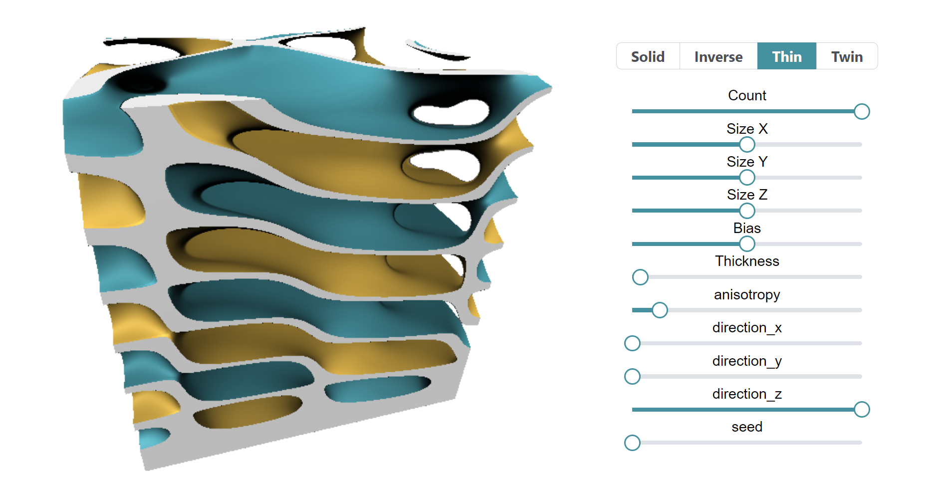
By observation in the 1D examples, the amplitude of our periodic fields is approximately half their period. We can think of starting with solid waveforms W(p) that can be biased by an initial offset:

Solid(p; bias) = W(p) - bias

and then create a thin-walled variant of it using the absolute value:

Thin(p; bias, thickness) = |W(p) - bias| - thickness/2

When our fields are defined by distance to already thin structures like beams, honeycomb, and foams, we model them as unsigned distance fields. Solid lattice become thin by taking their absolute value.

Note that there are many ways of combining 1D basis function into 3D fields, both periodic or not. For example, if you replace the three sine functions in the Schwarz equation above with with random but continuous functions, you get Perlin aka simplex noise (coming to LatticeRobot soon).

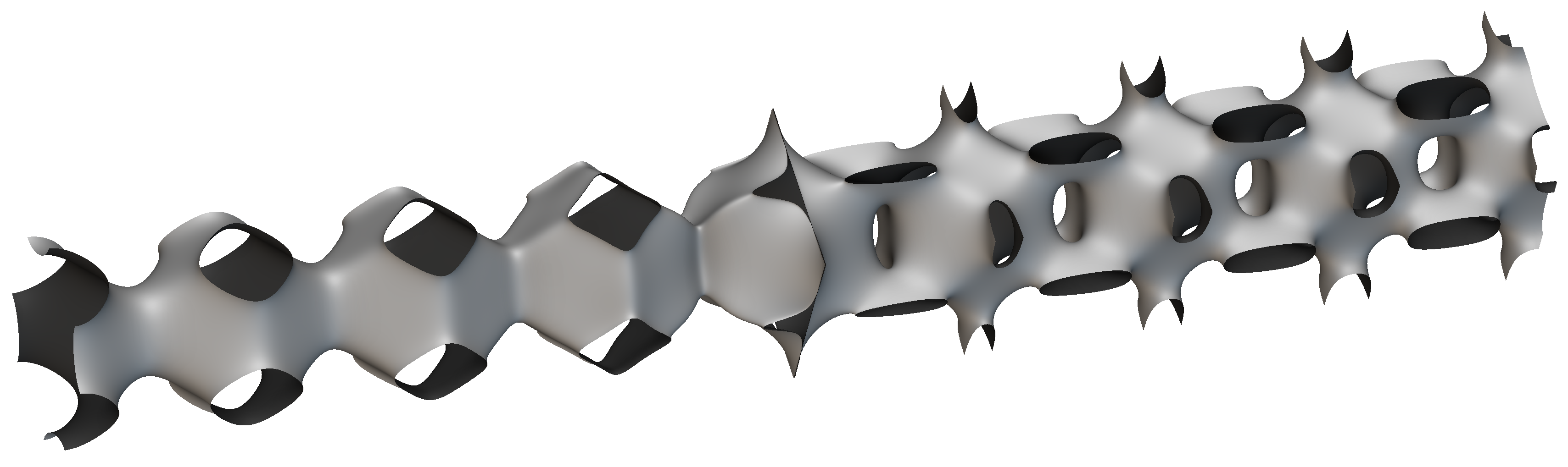
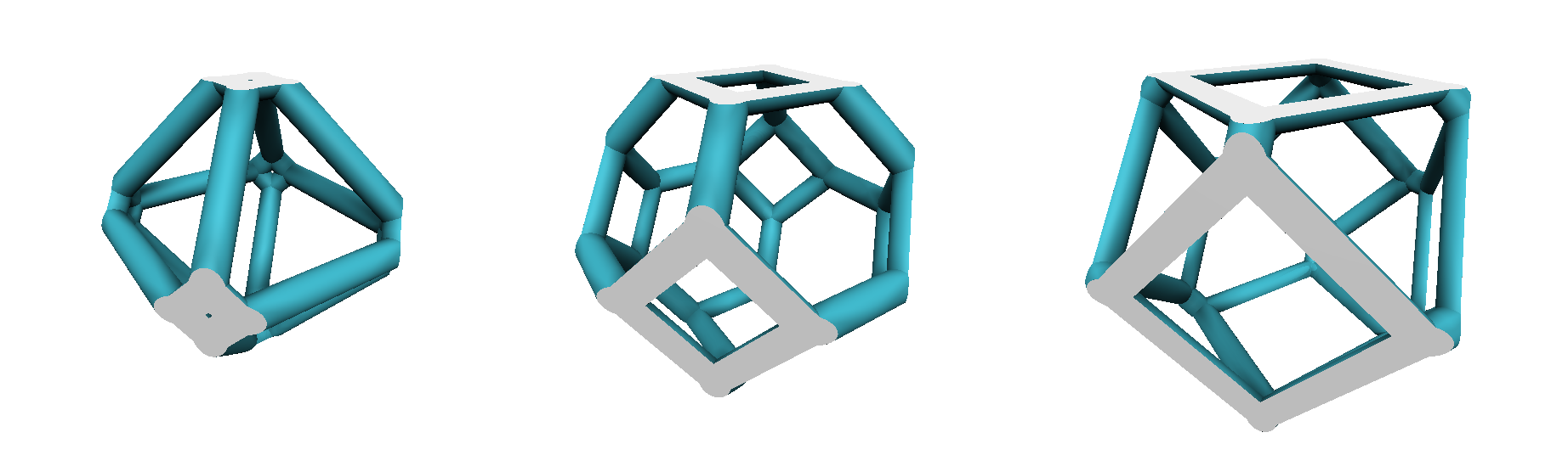
When making lattices, trig functions and triangle waves don't need to be constrained to the principle axes. The spinodal noise in the top image is the sum of many sine waves in many directions, modulated by the direction and anisotropy parameters.

Symmetry and Inverses

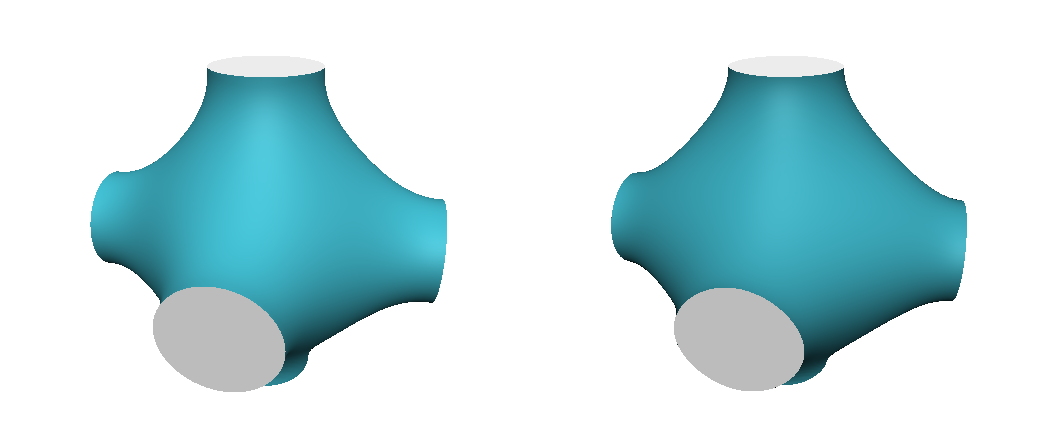
Many TPMS waveforms, such as the gyroid, diamond, and Schwarz, are congruent to their complements. You can take the negative of the function, transform it, and get back to the same shape. It's very much the 3D equivalent of the identity:

sin(x) = -sin(x - π)

However, most lattices are not complement-congruent, so let's define another variation of our waveform that produces the complementary structures:

Inverse(p; bias) = -Solid(p; bias)

To complete the picture, we can also invert the thin defined above to create a result with two disjoint regions. The result are the dual disconnected extrema of the field, and in the case of TPMS are known as its "twin axes":

Twin(p; bias, thickness) = -Thin(p; bias, thickness)

Although there are many more ways that fields such as TPMS and distance fields may be laminated into different domains, these four cases cover broad engineering applications and most of literature on lattice design.

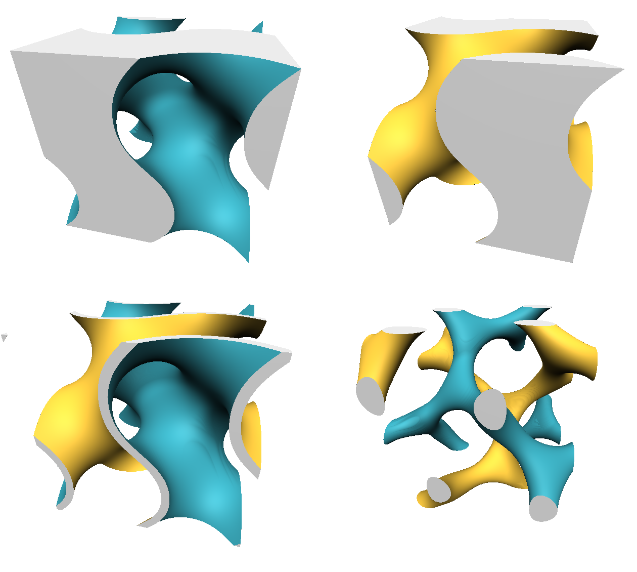
One other benefit is that when performing fluid simulation, we need to analyze the volume around the lattice, which is the inverse of the domain needed for structural and thermal simulation. This approach provides both to our simulation pipeline.

Symmetry and DOE complexity

When varying parameters to produce a design of experiments ("DOE"), the symmetry and range of the field can simplify the set of experiments needed. In particular, we follow these rules to reduce the DOE:

• The thickness parameter does not apply to Solid and Inverse variants.
• For complement-congruent fields, the Inverse variant is redundant, as is negative bias on Thin and Twin variants.
• For unsigned fields of thin geometry like beams, honeycombs, and foams, Solid and Inverse variants are redundant and for Thin, the thickness parameter behaves as expected. Note that blending unsigned fields may result in signed fields.

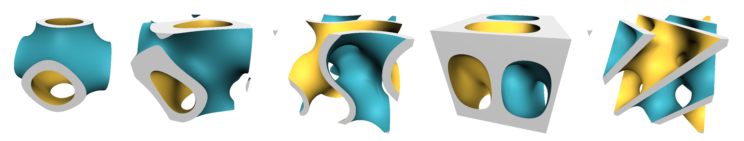
This approach does still have some collisions, as thin lattices with large bias can be the same as solid lattices with large bias. These parametric connections appear as coincident points in the Ashby plot, showing the connections of functional equivalence across disparate families.

Another way to understand these symmetries is through volume fraction plots, as designed in the recent TPMS survey by Joseph Fisher et al. Here are their plots for this Lidinoid TPMS:

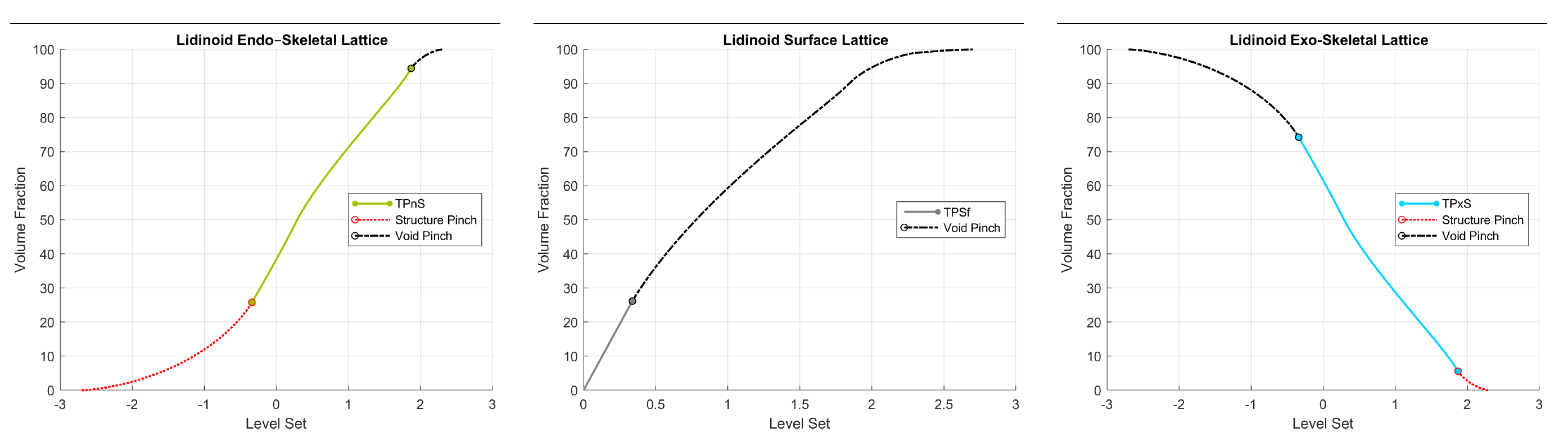
(Note: Fisher et al.'s level set parameter is equivalent to offset by the negative parameter and that the authors' definitions of endo-skeletal, surface, and exo-skeletal correspond to our concepts of Solid, Thin, and Inverse variants.)

Perhaps we'll add a similar plotting capability to LatticeRobot.

More Parameters

Many unit cells contain additional natural parameters. Classic TPMS theory shows that the minimal surfaces for gyroid, diamond, and Schwarz are parametrically related, and we can manipulate the terms of the TPMS functions to emulate those transitions more naturally than by simply interpolating the fields:

Similarly, we can zero out terms to lower the dimensionality of the TPMS periodicity, which can be useful for interfacing. Such is the purpose of the drop parameters on several of the lattices. For example, we enhance the Schwarz defined above with three new coefficients:

Schwarz(x, y, z) =
drop_x · cos(x) + drop_y · cos(y) + drop_z · cos(z)

We parameterize these drop_i in [-1, 1], with a default of 1. While 0 tends to flatten a dimension, -1 inverts it. In the case of Schwarz and many TPMS, negating the drop parameter inverts the phase of that dimension. In the case of a chiral structure like gyroid, it mirrors it:

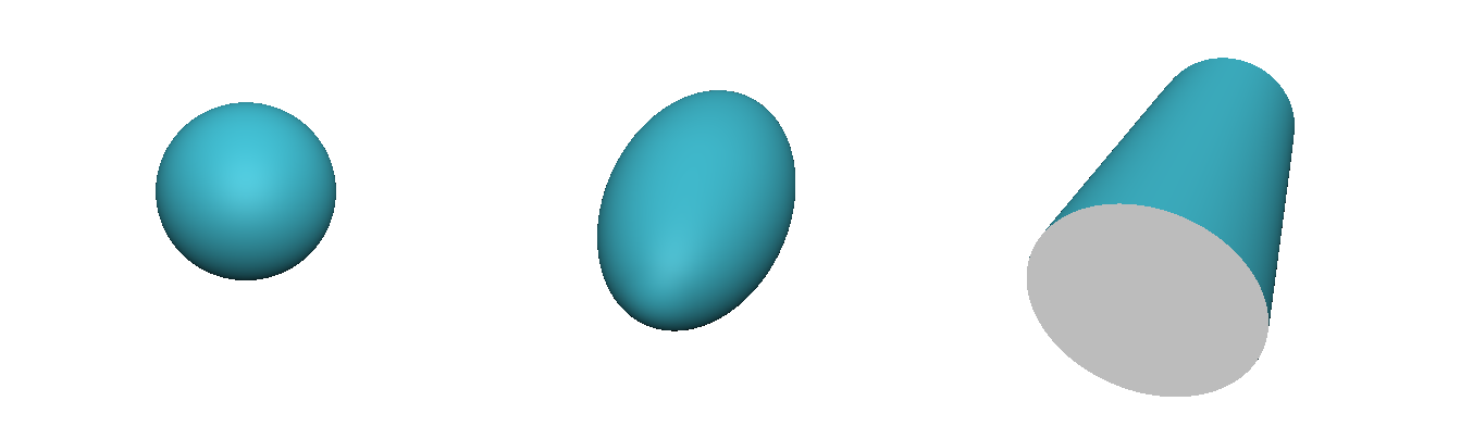
Another example is the drop parameter on a sphere:

Sphere(x, y, z) =
sqrt(drop_x · x² + drop_y · y² + drop_z · z²)

Which permits a transition from spheres to cylinders:

For explicit lattices like beams, there are often intermediate points like setbacks that present independent parameters:

Parameters may behavior differently across lattice families. For example, when changing the size of the unit cell, we stretch most cells or scale but with beams, we move the endpoint and preserve cylindricity.

The Relationship between Range and Period

Distance fields, and their generalization, unit gradient fields, have a predictable gradient with a gradient magnitude of 1. TPMS typically have varying gradient, but being periodic, and therefore finitely bounded, have well defined extrema. Can we use that information to reasonably scale the TPMS so they behave like distance fields and offset predictably?

Looking at the triangle wave in the example above, it's clear that the triangle wave, a distance field, has an amplitude of half the period. The sine curve is similar to the triangle wave to the extent that sin(x) ≈ x. If making thin-walled features, that approximation often works within manufacturing tolerance, but the appropriately scale extrema become ± period / (2 π). If one is most concerned about the behavior near the twin axes, scaling to period / (2 π) instead of period / 4 might be a better approximation of distance.

In LatticeRobot, we compute the extrema of the TPMS and scale to it, sacrificing gradient control at near the function's zero for predictable overall behavior. In the future, we may provide more tools for engineers who need to better control wall thickness.

Field-Parameterized Lattices for Everybody

To summarize, while the myriad lattices and their associated parameterizations are highly dimensional, patterns pervade their structures and connect them to each other both mathematically and functionally. At LatticeRobot, we're pairing reasonably sized parametric families of lattices with functional data to make both structures interactively explorable.

During this beta period, we look forward to your feedback on how we can make them more usable, both in LatticeRobot and your generative design tool of choice.